# Introduction

A lot of Prolog programming is about stating the obvious and having the system figure out the rest. This usually means writing facts and predicates that encode our knowledge of “the world”. However, sometimes what we know isn’t a universal fact, but a runtime invariant that can only be defined in the context of a predicate’s execution. In this article I want to demonstrate the usefulness of explicitly expressing some of those invariants at the code level.

Modern Prolog implementations provide an ability to attach constraints to variables before they are bound, through the primitive called attributed variables. These constraints can be conceptualized as expressing facts whose truthfulness is tied to a specific path of execution. They can also interact with each other, providing a way to inject non-local control into predicates. Here, I will present a technique that can considerably extend the power of structure-traversing predicates by using constraints to encode their invariants.

Code in this article uses clp(Z) library which is limited to integer values, but the principles can be applied beyond the domain of integers.

# List traversal

Suppose we’re using a predicate that matches elements of a list along with their indices. In SWI Prolog this is provided as the nth0 predicate.

If we wish to find only elements between positions N and M , we may use it like this:

nth0(Index, List, Elem),
N =< Index, Index < M,

This code works, but it needlessly iterates over all elements of the list, even though everything past the M-th one will be discarded. The complexity of this code is thus $O(|List|)$. The problem lies in that Index is tested too late to avoid this unnecessary work.

A naive solution would be to first iterate over Index like so:

between(N, M, Index),
nth0(Index, List, Elem),

This avoids iterating over the irrelevant tail of the list, but instead traverses the list up to each element separately, producing a potentially even worse complexity of $O(M^2)$. Clearly the iteration must come from back-tracking inside the nth0 predicate if we want to avoid the issue above.

We could introduce a cut after testing for Index > M, but this can be undesirable if we want to preserve purity of our code. Another approach would be to implement a predicate nth0_before taking limit M as an additional parameter, but this means that we now have two predicates with almost identical implementations to maintain, one of which is of quite specific use.

As it turns out, we can implement our own version of nth0 - elem_at - that can avoid this problem:

elem_at(Index, List, Elem) :-
    elem_at_inner(Index, 0, List, Elem).
elem_at_inner(Index, Index, [Elem | _], Elem).
elem_at_inner(Index, IndexCandidate, [_ | Rest], Elem) :-
    Index #> IndexCandidate,
    NewIndexCandidate #= IndexCandidate + 1,
    elem_at_inner(Index, NewIndexCandidate, Rest, Elem).

This is similar to what nth0’s (simplified) implementation could look like, but notice that in the recursive case we assert that Index #> IndexCandidate. This assertion is not necessary for elem_at to work correctly; instead its function is to express an invariant, which we already know holds, explicitly in a way that can be used at runtime. It uses the #> predicate coming from the clp(Z) library which, in contrast to Prolog’s inbuilt > comparison used in previously shown bound checks, doesn’t run immediately when called. Instead, it registers a constraint on the variables Index and IndexCandidate.

Now, to find elements between N and M we may write the following:

N #=< Index, Index #< M,
elem_at(Index, Elem, List),

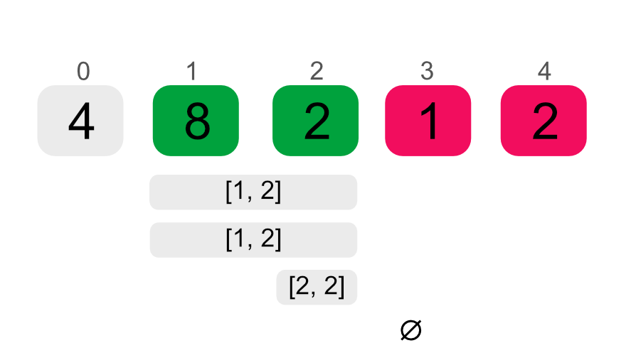
This code is similar to the one using between, but here we are using #=< and #<, introducing a constraint on Index instead of directly iterating over the desired indices. When elem_at is run, this constraint is further narrowed down by being combined with Index #> IndexCandidate and once IndexCandidate internally passes the value of M, elem_at will finish without traversing the rest of the list.

This example is interesting, but ultimately there are much better ways to achieve the same result. We could simply drop N and then take M - N elements. The performance gain is highly dependent on M and the length of List. Nevertheless, we achieved the asymptotically optimal complexity of $O(M)$ at the cost of introducing a bigger constant.

The same technique can also be applied to more complex structures where it makes a little bit more sense.

# Binary tree traversal

Suppose we are working with integer-valued binary search trees of the following structure:

tree --> nil | node(Left, Value, Right) 

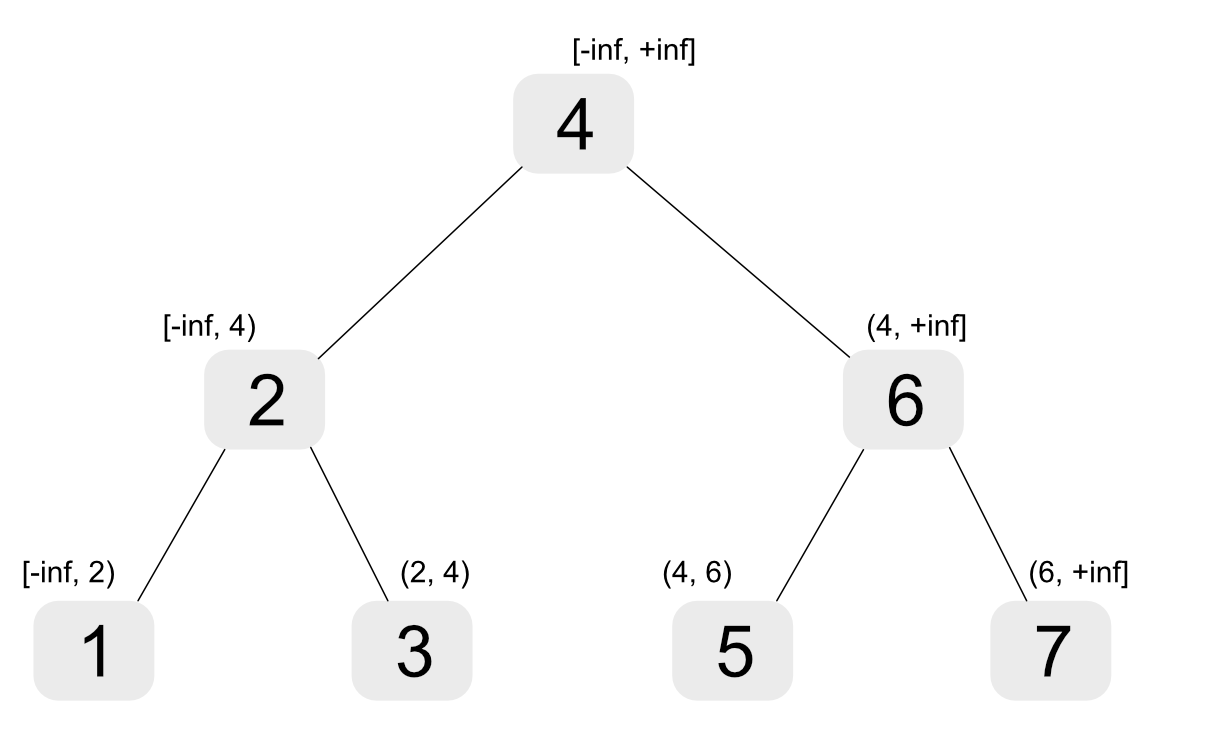
The invariant here is that values in Left are less or equal to Value while those in Right are greater or equal to it.

We can implement a predicate like the following, that simply traverses all elements of a tree in order:

tree_elem(node(Left, NodeValue, _), Value) :-
    Value #=< NodeValue, 	
    tree_elem(Left, Value).
tree_elem(node(_, Value, _), Value). 
tree_elem(node(_, NodeValue, Right), Value) :- 	
    NodeValue #=< Value,
    tree_elem(Right, Value).

Again, we’ve introduced constraints on a variable - this time on the value as opposed to its index - which is not necessary for the predicate’s correctness. However, like in the previous example, it allows us to narrow down the results to a specific range:

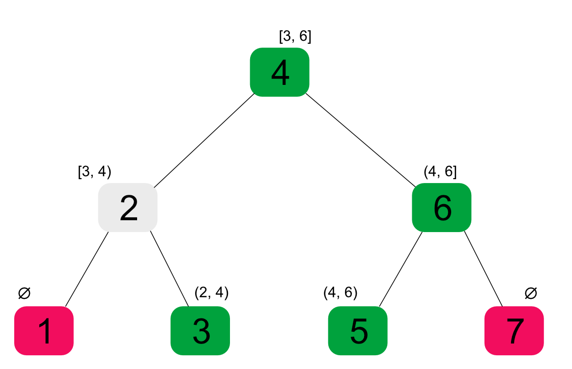
5 #< Value, Value #< 12,
tree_elem(Tree, Value),

Not only does the code correctly find the values within the specified range, but it also visits just the nodes that are necessary to do it. The way it works, is that the constraint on Value always corresponds to the range of acceptable values that could be present within the current sub-tree.

This means that at the cost of two additional lines of code our simple in-order traversal predicate can now also be used to query the tree’s data in multiple ways, and does so in an asymptotically optimal way. Compared to the list traversal example, this predicate might actually be of practical use. Also note, that as long as Value is exposed from the predicate that calls tree_elem, the ability to inject constraints this way can also be made part of its API.

# Other uses and final thoughts

It’s probably clear, that this technique can be applied in more cases. Possible ideas include:

• tree traversal depth - limiting search depth, querying elements at particular depth
• list element counting - finding N-th to M-th matching elements
• constraining graph path weights

The key requirement is that some monotonic invariant is identified for which an applicable constraint system exists. The examples in this article all used numeric constraints, but monotonicity in other domains (eg. over term structure) could be explored.

This article talked about constraints where a value was within a signle interval for simplicity, but both predicates shown here retain their correctness and performance characteristics for any clp(Z) constraint set (ie. discontiguous sum of intervals).

However, when performance is a concern, it must be noted that using constraints like that introduces some overhead that can be avoided with a bespoke implementation, especially for cases where the constraint is unneeded.

At the same time it must be appreciated that from a user’s point of view, predicates written in this way provide good ergonomics and readability, compared to special-purpose predicates. They also don’t introduce too much complexity for the maintainers, in proportion to the extension of functionality offered.